Fundamental plane-source similarity solution

Your work doesn't need to be as detailed as this.

Source code for the (non-hand-drawn) images: code.wl
Return to the home page.

Problem

Consider an infinite, uniform block of thermal conductivity k, density \rho, and specific heat capacity c. Its thermal diffusivity is therefore \kappa = k / (\rho c).

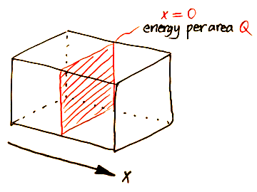
Suppose the block is initially at zero temperature throughout. At time t = 0:

What happens?

Diagram for fundamental plane-source problem

Q. How can you put a non-zero amount of thermal energy into a plane which has zero thickness?
A. It's an idealisation, like a point charge. In the case of a point charge, the charge density is infinite but the amount of charge is finite. Here, the initial temperature of the plane x = 0 will be infinite, but the energy per area is finite.

Quantities

We find that by defining

Q' = \frac{Q}{\rho c},

the equations for this problem can be written in terms of the constants \kappa and Q' only (rather than k, \rho, c, and Q). Note that Q' is to Q as \kappa is to k.

Independent variables
x position (-\infty < x < \infty)
t time (t \ge 0)
Dependent variable
T temperature
Constants
\kappa thermal diffusivity
Q' initial energy per area divided by \rho c

Defining equations

Partial differential equation (PDE)

Heat equation in T = T (x, t), throughout the block, for all time:

\frac{\pd T}{\pd t} = \kappa \frac{\pd^2 T}{{\pd x}^2}

Boundary condition (BC)

Nothing happens at (spatial) infinity, for all time:

\eval{T}_{x = \pm\infty} = 0

If you prefer limit notation: \lim_{x \to \pm\infty} T (x, t) = 0.

Initial condition (IC)

\gdef \dimen #1 {\textsf{#1}}

All of the thermal energy is concentrated in the slice x = 0, initially:

\eval{T}_{t = 0} = \begin{cases} \infty, & x = 0 \\ 0, & x \ne 0 \end{cases}

If you prefer limit notation: \lim_{t \to 0^+} T (x, t) = \footnotesize \left\{ \begin{matrix} \infty, & x = 0 \\ 0, & x \ne 0 \end{matrix} \right..

Q. What nonsense is this?
A. The formal way to write this initial condition is
\eval{T}_{t = 0} = Q' \cdot \delta (x).
The Q' factor arises from the conservation of energy condition.

Here \delta (x) is the unit impulse or Dirac delta function. (Mathematicians prefer to call it a "generalised function" or a "distribution".) Basically \delta (x) is zero everywhere except at x = 0, where it is infinity, in such a way that the area under the curve is 1:

\begin{gathered} \delta (x) = \begin{cases} \infty, & x = 0 \\ 0, & x \ne 0 \end{cases} \\ \int_{-\infty}^\infty \delta (x) \td x = 1 \end{gathered}
The easiest way to think of \delta (x) is as a normal distribution with a standard deviation of zero, or as an infinitely tall and thin spike with area 1. Note that \delta (x) has dimensions of 1 / \dimen{Length}.

Conservation of energy

Energy is conserved, for all time:

\int_{-\infty}^\infty T \td x = Q'
Q. Why is the right hand side Q'?
A. The initial injection has energy per area Q in the plane x = 0. In other words if we take a portion of that plane with area A, the total energy within that portion will be Q A.

Subsequently the energy will spread out in the x-direction, but since energy is conserved, if we take an infinite cylinder (aligned with the x-axis) with cross-sectional area A, the total energy within that cylinder will still be Q A.

Now recall that \textq{Energy} = m c \textq{Temperature}. Therefore the energy in the cylinder is

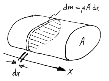
Q A = \int c T \td m.
Slice of the cylinder of thickness dx
Taking each mass element to be a slice of thickness \td x, the differential mass is \td m = \rho A \td x. Therefore
Q A = \int_{-\infty}^\infty c T \rho A \td x,
or
\int_{-\infty}^\infty T \td x = \frac{Q}{\rho c} = Q'.

Summary

That was a lot to process, so here are the defining equations again without the commentary:

\begin{aligned} \frac{\pd T}{\pd t} &= \kappa \frac{\pd^2 T}{{\pd x}^2} \\[\tallspace] \eval{T}_{x = \pm\infty} &= 0 \\ \eval{T}_{t = 0} &= \begin{cases} \infty, & x = 0 \\ 0, & x \ne 0 \end{cases} \\ \int_{-\infty}^\infty T \td x &= Q' \end{aligned}

Scaling

Normally there will be a length scale provided by the parameters. But in the current situation the only parameters are \kappa and Q', and:

Both infinity and zero are scale-invariant. THERE IS NO LENGTH SCALE.

Q. So how do we scale x?
A. Somehow a combination of the other quantities t, \kappa, and Q' must form a length scale to compare against x.

Dimensional analysis

\gdef \termnote #1 #2 {\underbrace{#1}_{\substack{\small #2}}} \gdef \termnotetext #1 {\footnotesize \text{#1}} \gdef \temp #1 {\colg{#1}} \gdef \dimenless #1 {\colv{#1}}

The temperature T can only depend on the independent variables x and t and the constants \kappa and Q', because there are no other variables or physical constants in the defining equations:

T = T (x, t; \kappa, Q')

The only way this can make dimensional sense is if

T = \temp{\mathcal{T}} \cdot \dimenless{\mathcal{L}},

where \temp{\mathcal{T}} is a combination (of x, t, \kappa, and Q') which has dimensions of temperature, and \dimenless{\mathcal{L}} is a combination which is dimensionless.

Obviously

\begin{aligned} [T] &= \dimen{Temp} \\ [x] &= \dimen{Length} \\ [t] &= \dimen{Time}. \end{aligned}

From the PDE, we have

[\kappa] = \frac{\dimen{Length}^2}{\dimen{Time}},

and from the conservation of energy condition, we see that

[Q'] = \dimen{Temp} \cdot \dimen{Length}.

You should be able to show that

\begin{aligned} \squarebr{\temp{\frac{Q'}{\sqrt{\kappa t}}}} &= \temp{\dimen{Temp}} \\ \squarebr{\dimenless{\frac{x}{\sqrt{\kappa t}}}} &= \dimenless{\dimen{1}}. \end{aligned}

Therefore T must be of the form

T = \temp{\frac{Q'}{\sqrt{\kappa t}}} \cdot U \roundbr{\dimenless{\frac{x}{\sqrt{\kappa t}}}},

where U is some dimensionless function. We give the dimensionless group a name:

\dimenless{\xi} = \dimenless{\frac{x}{\sqrt{\kappa t}}}
Q. Is there a systematic way of doing this?
A. Yes, read up on the Buckingham pi theorem.
In the present scenario, suppose that
\gdef \ind #1 {\colr{#1}} [T] = [x]^{\ind{p}} [t]^{\ind{q}} [\kappa]^{\ind{r}} [Q']^{\ind{s}}
for some indices \ind{p}, \ind{q}, \ind{r}, and \ind{s}. Then
\dimen{Temp} = \dimen{Length} ^ {\ind{p}} \cdot \dimen{Time} ^ {\ind{q}} \roundbr{\frac{\dimen{Length}^2}{\dimen{Time}}} ^ {\ind{r}} \roundbr{\dimen{Temp} \cdot \dimen{Length}} ^ {\ind{s}}.
Equating powers of \dimen{Length}, \dimen{Time}, and \dimen{Temp}, we get the system of linear equations
\begin{aligned} \ind{p} + 2 \ind{r} + \ind{s} &= 0 \\ \ind{q} - \ind{r} &= 0 \\ \ind{s} &= 1, \end{aligned}
which solves to give
\begin{pmatrix} \ind{p} \\ \ind{q} \\ \ind{r} \\ \ind{s} \end{pmatrix} = \termnote{ \begin{pmatrix} 0 \\ -1/2 \\ -1/2 \\ 1 \end{pmatrix} }{ \temp{Q' / \sqrt{\kappa t}} } + a \termnote{ \begin{pmatrix} 1 \\ -1/2 \\ -1/2 \\ 0 \end{pmatrix} }{ \dimenless{x / \sqrt{\kappa t}} },
where a is a free variable. Thus we obtain the temperature combination \temp{Q' / \sqrt{\kappa t}} and the dimensionless group \dimenless{x / \sqrt{\kappa t}}.

Change of coordinates

\gdef \old #1 {\colb{#1}} \gdef \new #1 {\colr{#1}}

The result of the dimensional analysis says that we should move from (x, t) coordinates with dependent variable T, i.e.

T (\old{x}, \old{t}) = \frac{Q'}{\sqrt{\kappa \old{t}}} \cdot U \roundbr{\frac{\old{x}}{\sqrt{\kappa \old{t}}}}

to (\xi, t) coordinates with dependent variable U, i.e.

T (\new{\xi}, \new{t}) = \frac{Q'}{\sqrt{\kappa \new{t}}} \cdot U (\new{\xi}).

To do this, we will need the chain rule:

Chain rule

Suppose the change of coordinates from old coordinates (x, y) to new coordinates (r, s) is given by

\begin{aligned} \new{r} &= \old{r (x, y)} \\ \new{s} &= \old{s (x, y)}. \end{aligned}

Then the chain rule says that the partial derivatives will transform thus:

\begin{aligned} \old{\frac{\pd}{\pd x}} &= \old{\frac{\pd r}{\pd x}} \new{\frac{\pd}{\pd r}} + \old{\frac{\pd s}{\pd x}} \new{\frac{\pd}{\pd s}} \\[\tallspace] \old{\frac{\pd}{\pd y}} &= \old{\frac{\pd r}{\pd y}} \new{\frac{\pd}{\pd r}} + \old{\frac{\pd s}{\pd y}} \new{\frac{\pd}{\pd s}} \end{aligned}

It is vital that you understand what the chain rule means, and not just what it says. Let us unpack the meaning:

\begin{aligned} \termnote{ \old{\frac{\pd}{\pd x}} }{ \termnotetext{Derivative} \\ \termnotetext{w.r.t. $\old{x}$}, \\ \termnotetext{with $\old{y}$ held} \\ \termnotetext{constant} } &= \termnote{ \old{\frac{\pd r}{\pd x}} }{ \termnotetext{Derivative} \\ \termnotetext{of $\old{r (x, y)}$} \\ \termnotetext{w.r.t. $\old{x}$}, \\ \termnotetext{with $\old{y}$ held} \\ \termnotetext{constant} } \cdot \termnote{ \new{\frac{\pd}{\pd r}} }{ \termnotetext{Derivative} \\ \termnotetext{w.r.t. $\new{r}$}, \\ \termnotetext{with $\new{s}$ held} \\ \termnotetext{constant} } + \termnote{ \old{\frac{\pd s}{\pd x}} }{ \termnotetext{Derivative} \\ \termnotetext{of $\old{s (x, y)}$} \\ \termnotetext{w.r.t. $\old{x}$}, \\ \termnotetext{with $\old{y}$ held} \\ \termnotetext{constant} } \cdot \termnote{ \new{\frac{\pd}{\pd s}} }{ \termnotetext{Derivative} \\ \termnotetext{w.r.t. $\new{s}$}, \\ \termnotetext{with $\new{r}$ held} \\ \termnotetext{constant} } \\[6em] \termnote{ \old{\frac{\pd}{\pd y}} }{ \termnotetext{Derivative} \\ \termnotetext{w.r.t. $\old{y}$}, \\ \termnotetext{with $\old{x}$ held} \\ \termnotetext{constant} } &= \termnote{ \old{\frac{\pd r}{\pd y}} }{ \termnotetext{Derivative} \\ \termnotetext{of $\old{r (x, y)}$} \\ \termnotetext{w.r.t. $\old{y}$}, \\ \termnotetext{with $\old{x}$ held} \\ \termnotetext{constant} } \cdot \termnote{ \new{\frac{\pd}{\pd r}} }{ \termnotetext{Derivative} \\ \termnotetext{w.r.t. $\new{r}$}, \\ \termnotetext{with $\new{s}$ held} \\ \termnotetext{constant} } + \termnote{ \old{\frac{\pd s}{\pd y}} }{ \termnotetext{Derivative} \\ \termnotetext{of $\old{s (x, y)}$} \\ \termnotetext{w.r.t. $\old{y}$}, \\ \termnotetext{with $\old{x}$ held} \\ \termnotetext{constant} } \cdot \termnote{ \new{\frac{\pd}{\pd s}} }{ \termnotetext{Derivative} \\ \termnotetext{w.r.t. $\new{s}$}, \\ \termnotetext{with $\new{r}$ held} \\ \termnotetext{constant} } \end{aligned}

Especially take note of what variable is held constant in each partial derivative, because:

Ambiguity

In the current problem, the time coordinate t appears in both the old and the new coordinate systems. We need to be VERY careful, because \pd /{\pd t} is ambiguous:

These are NOT the same thing.

To disambiguate between the two possible meanings of \pd /{\pd t}, it is common to use subscripts to indicate which variable is being held constant:

Changing coordinates

Let us CAREFULLY apply the change of coordinates now. The coordinate transformation is given by

\begin{aligned} \new{\xi} &= \frac{\old{x}}{\sqrt{\kappa \old{t}}} \\ \new{t} &= \old{t}. \end{aligned}

After a lot of algebra, the chain rule equations become

\begin{aligned} \old{\frac{\pd}{\pd x}} &= \frac{1}{\sqrt{\kappa \new{t}}} \new{\frac{\pd}{\pd\xi}} \\[\tallspace] \old{\roundbr{\frac{\pd}{\pd t}}_x} &= -\frac{\new{\xi}}{2 \new{t}} \new{\frac{\pd}{\pd\xi}} + \new{\roundbr{\frac{\pd}{\pd t}}_\xi}. \end{aligned}

We then apply the 1st of these twice, and the 2nd of these once, to the equation

T (\old{x}, \old{t}) = \frac{Q'}{\sqrt{\kappa \new{t}}} \cdot U (\new{\xi}).

After a lot of algebra, this gives us

\begin{aligned} \old{\frac{\pd^2 T}{{\pd x}^2}} &= \frac{Q'}{(\kappa \new{t}) ^ {3/2}} \frac{\new{\td^2} U}{\new{{\td \xi}^2}} \\[\tallspace] \old{\roundbr{\frac{\pd T}{\pd t}}_x} &= - \frac{\new{\xi}}{2 \new{t}} \frac{Q'}{\sqrt{\kappa \new{t}}} \frac{\new{\td} U}{\new{\td \xi}} + \frac{Q'}{\sqrt{\kappa}} \cdot \frac{-1/2}{\new{t} ^ {3/2}} \cdot U. \end{aligned}

Finally, substituting these into the heat equation, we obtain (after a little algebra)

\frac{\new{\td^2} U}{\new{{\td \xi}^2}} + \frac{\new{\xi}}{2} \frac{\new{\td} U}{\new{\td \xi}} + \frac{U}{2} = 0.

Thus we have reduced the PDE to an ODE.

Change of coordinates for the boundary/initial conditions

If you stare at the equations

\begin{aligned} T (\old{x}, \old{t}) &= \frac{Q'}{\sqrt{\kappa \new{t}}} \cdot U (\new{\xi}) \\ \frac{\old{x}}{\sqrt{\kappa \old{t}}} &= \new{\xi} \end{aligned}

for long enough, you will see that the condition

\eval{U}_{\new{\xi} = \pm\infty} = 0

(or \lim_{\new{\xi} \to \pm\infty} U (\new{\xi}, \new{t}) = 0 if you prefer limit notation) takes care of both the boundary condition and the initial condition.

Change of coordinates for conservation of energy

Writing the integral condition for conservation of energy backwards, we have

\begin{aligned} Q' &= \int_{-\infty}^\infty T \td \old{x} \\[\tallspace] &= \int_{-\infty}^\infty \frac{Q'}{\sqrt{\kappa \new{t}}} \cdot U (\new{\xi}) \td \old{x} \\[\tallspace] &= \int_{\old{x} = -\infty} ^ {\old{x} = \infty} Q' \cdot U (\new{\xi}) \td \roundbr{\frac{\old{x}}{\sqrt{\kappa \old{t}}}}, \end{aligned}

where \old{t} is held constant for the purposes of evaluating the integral. Now \new{\xi} = \old{x} / \sqrt{\kappa \old{t}}. With \old{t} held constant and \old{x} running from -\infty to \infty, the variable \new{\xi} will also run from -\infty to \infty. Therefore

Q' = \int_{\new{\xi} = -\infty} ^ {\new{\xi} = \infty} Q' \cdot U (\new{\xi}) \td \new{\xi},

i.e.

\int_{-\infty}^\infty U (\new{\xi}) \td\new{\xi} = 1.

Solution to the ODE

To recap, we have reduced the problem to an ODE, an associated boundary condition, and an integral condition:

\begin{gathered} \frac{\new{\td^2} U}{\new{{\td \xi}^2}} + \frac{\new{\xi}}{2} \frac{\new{\td} U}{\new{\td \xi}} + \frac{U}{2} = 0 \\[\tallspace] \eval{U}_{\new{\xi} = \pm\infty} = 0 \\[\tallspace] \int_{-\infty}^\infty U (\new{\xi}) \td\new{\xi} = 1 \end{gathered}

Use Mathematica to solve the ODE:

DSolveValue[u''[xi] + xi/2 * u'[xi] + u[xi]/2 == 0, u[xi], xi]

This gives the linearly independent solutions

\gdef \erfi {\operatorname{erfi}} \gdef \Uodd {U_\mathrm{odd}} \gdef \Ueven {U_\mathrm{even}} \begin{aligned} \Uodd &= \sqrt{\pi} \exp \frac{-\xi^2}{4} \erfi \frac{\xi}{2} \\[\tallspace] \Ueven &= \exp \frac{-\xi^2}{4}, \end{aligned}

where \erfi is the imaginary error function.

Odd and even solutions to the ODE

There are several reasons why \Uodd does not work for the plane-source problem:

Therefore the solution must consist of the even term only, i.e.

U (\new{\xi}) = C \exp \frac{-\new{\xi}^2}{4}.

The constant C is determined by the integral condition, which becomes

\int_{-\infty}^\infty C \exp \frac{-\new{\xi}^2}{4} \td\new{\xi} = 1,

giving

C = \left. 1 \middle/ \int_{-\infty}^\infty \exp \frac{-\new{\xi}^2}{4} \td\new{\xi} \right. = \frac{1}{2 \sqrt{\pi}}

courtesy of Mathematica:

1 / Integrate[Exp[-xi^2 / 4], {xi, -Infinity, Infinity}]

Therefore:

U (\new{\xi}) = \frac{1}{2 \sqrt{\pi}} \exp \frac{-\new{\xi}^2}{4}.

Result

Putting everything together, the fundamental plane-source similarity solution is

T (\new{\xi}, \new{t}) = \frac{Q'}{\sqrt{\kappa \new{t}}} \cdot \frac{1}{2 \sqrt{\pi}} \exp \frac{-\new{\xi}^2}{4}

and therefore

T (\old{x}, \old{t}) = \frac{Q'}{2 \sqrt{\pi \kappa \old{t}}} \exp \frac{-\old{x}^2}{4 \kappa \old{t}}.

Note that the solution profile T (x, t) has

so for small t it is a tall, thin spike (corresponding to heat concentrated near x = 0) and for large t it flattens out to a broad bump.

At all times the area under the curve is Q' (see conservation of energy).

Visualising the solution

Since the similarity solution is scale-invariant, in order to plot the solution we need to introduce an arbitrary length scale. Calling the length scale x_0, we define the dimensionless variables

\begin{aligned} x' &= x / x_0 \\ t' &= \kappa t / {x_0}^2 \\ T' &= x_0 T / Q'. \end{aligned}

Substituting these, we get

T' (x', t') = \frac{1}{2 \sqrt{\pi t'}} \exp \frac{-{x'}^2}{4 t'}.

Having removed the parameters \kappa and Q', we can now plot the solution:

Animation of temperature profile

END

Return to the home page.