Single-lane traffic model

Source code for images: code.wl
Return to the home page.

This page summarises the simple continuum model for single-lane traffic. For some cool animations, see the following:

• Light change example
• Pile up example

Curves for the simple model

Speed vs density

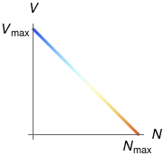
With the exception of tailgaters, drivers tend to go slower when the traffic is denser. The simplest model is a linear relationship between the density N (amount of vehicle per length of road) and the preferred speed V:

• When there is no traffic (N = 0), drivers will go at the speed limit (V = \Vmax).
• When there is bumper-to-bumper traffic (N = \Nmax), drivers will halt (V = 0).

We also assume that drivers are able to adjust their speed instantly when the density changes. This might not seem realistic, but remember we are constructing a model. (Also note that in real life, most drivers are happy to do the speed limit even when the density isn't zero, by keeping at a 2-second separation to the vehicle ahead.)

Flux vs density

Traffic engineers generally want to maximise the flux of traffic, which is the product of density and speed:

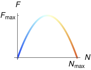
In our current model this is a parabolic relationship:

• Maximum flux \Fmax = \Nmax \Vmax / 4 is obtained with traffic at half the maximum density going at half the speed limit.
• The flux is zero in both the empty-street case N = 0, V = \Vmax (because there are no cars) and in the bumper-to-bumper case N = \Nmax, V = 0 (because the cars aren't moving).

Note that there are two ways to achieve a given flux F < \Fmax: fast & sparse, and slow & dense (with the former being preferable to drivers).

Traffic equation

Quantities

Conservation

After doing the usual conservation analysis (here, "conservation of vehicle"), we obtain the continuity equation

and since we have a direct relationship F = F (N) between flux and density, this becomes the traffic equation

Signal speed

The quantity \td F / {\td N} has dimensions of speed, and varies linearly from +\Vmax at zero density to -\Vmax at maximum density:

It turns out that \td F / {\td N} is the signal speed for the local density:

Method of characteristics

Unlike the heat equation, the traffic equation is a hyperbolic PDE. Instead of separation of variables, we use the method of characteristics.

We seek characteristic curves x = \xc (t) along which the density N (x, t) is constant, i.e.

By definition \td N = 0 along a characteristic, and using the chain rule we have

Comparing this with the traffic equation

we see that the characterstics are given by

Thus the characteristics are straight lines in spacetime with slope equal to the signal speed \td F / {\td N}.

Note that characteristics are NOT the trajectories of the cars; they are curves along which density is constant.

Steps

Given a traffic problem:

1. Draw a spacetime diagram with position x on the horizontal axis and time t on the vertical axis.
2. Mark the locations in spacetime where the density N is given by the boundary and initial conditions.
3. For a bunch of these locations:
   1. Work out the signal speed \td F / {\td N} for the given value of N.
   2. Draw the associated characteristic curve through this location (the straight line with slope \td F / {\td N}).

Since characteristics are curves with constant density N, this procedure "extends" the boundary/initial values of N to all of spacetime. In other words, we've solved for N (x, t). That's all there is to do.

If we wanted to find the actual trajectories x = x (t) of the cars, we would:

1. Determine V (x, t) from N (x, t) using the speed vs density relationship.
2. Solve the ODE \td x / {\td t} = V (x, t). We could also proceed graphically; simply sketch the trajectories so that the slope (which is the speed) matches V (x, t).

Finally, since time is on the vertical axis, remember that "fast" trajectories are near-horizontal while "slow" trajectories are near-vertical.

Examples:

• Light change example
• Pile up example

Return to the home page.